Category: Coding

Topics related to software development

Integrating Rmathlib and kdb+

Post author By Rory Winston
Post date January 9, 2013

The R engine is usable in a variety of ways – one of the lesser-known features is that it provides a standalone math library that can be linked to from an external application. This library provides some nice functionality such as:

* Probability distribution functions (density/distribution/quantile functions);
* Random number generation for a large number of probability distributions

In order to make use of this functionality from q, I built a simple Rmathlib wrapper library. The C wrapper can be found here and is simply a set of functions that wrap the appropriate calls in Rmathlib. For example, a function to generate N randomly-generated Gaussian values using the underlying rnorm() function is:

K rnn(K n, K mu, K sigma) {
int i,count = n->i;
K ret = ktn(KF, count);
for (i = 0; i < count; ++i)
kF(ret)[i] = rnorm(mu->f, sigma->f);
return ret;
}

These have to be imported and linked from a kdb+ session, which is done using special directives (the 2: verb). I decided to automate the process of generating these directives – the code shell script below parses a set of function declarations in a delimited section of a C header file and produces the appropriate load statements:

INFILE=rmath.h
DLL=\`:rmath

echo "dll:$DLL"

DECLARATIONS=$(awk '/\/\/ BEGIN DECL/ {f=1;next} /\/\/ END DECL/ {f=0} f {sub(/K /,"",$0);print $0}' $INFILE)
for decl in $DECLARATIONS; do
FNAME=${decl%%(*}
ARGS=${decl##$FNAME}
IFS=, read -r -a CMDARGS <<< "$ARGS"
echo "${FNAME}:dll 2:(\`$FNAME;${#CMDARGS[*]})"
done

echo "\\l rmath_aux.q"

This generates a set of link commands such as the following:

dll:`:rmath
rn:dll 2:(`rn;2)
rnn:dll 2:(`rnn;3)
dn:dll 2:(`dn;3)
pn:dll 2:(`pn;3)
qn:dll 2:(`qn;3)
sseed:dll 2:(`sseed;2)
gseed:dll 2:(`gseed;1)
nchoosek:dll 2:(`nchoosek;2)

It also generates a call to load a second q script, rmath_aux.q, which contains a bunch of q wrappers and helper functions (I will write a separate post about that later).

A makefile is included which generates the shared lib (once the appropriate paths to the R source files is set) and q scripts. A sample q session looks like the following:

q) \l rmath.q q) x:rnorm 1000 / generate 1000 normal variates q) dnorm[0;0;1] / normal density at 0 for a mean 0 sd 1 distribution

The project is available on github: https://github.com/rwinston/kdb-rmathlib.

Note that loading rmath.q loads the rmath dll, which in turn loads the rmathlib dll, so the rmathlib dll should be available on the dynamic library load path.

[Check out Part 2 of this series]

Coding kdb R

Exporting Data From R to KDB

Post author By Rory Winston
Post date December 12, 2012

Here is the beginnings of a simple routine to convert R data frames to Q format (in this case a dictionary). It uses the S3 dispatch mechanism to handle the conversion of different data types. Extremely basic (I havent even bothered to put in proper file output – just capturing the output of cat) but very quick to knock up.

The code is mainly a top-level function called to_dict:

[code lang=”R”]
to_dict <- function(x) {
cat(substitute(x),":", sep="")
nms <- names(x)
for (n in nms) { cat("`",n,sep="") }
cat("!(",sep="")
r <- rep(c(";",")"),times=c(length(nms)-1,1))
for (i in 1:length(nms)) { cat(qformat(x[[nms[i]]]),r[i],sep="") }
}
[/code]

Where qformat is a generic S3 function:

[code lang=”R”]
qformat <- function(x) {
UseMethod("qformat")
}

qformat.default <- function(x) {
cat("",format(x))
}

qformat.logical <- function(x) {
cat(ifelse(x==TRUE,"1b","0b"))
}

qformat.factor <- function(x) {
cat("",gsub("\\s","",format(x)), sep="`")
}
[/code]

It can be used as follows (using the famous Anscombe quartet data):

[code lang=”R”]
> write(capture.output(to_dict(anscombe)),
file="/tmp/anscombe.q")
[/code]

Then within a Q session:

q)\l /tmp/anscombe.q
q)anscombe
x1| 10 8 13 9 11 14 6 4 12 7 5
x2| 10 8 13 9 11 14 6 4 12 7 5
x3| 10 8 13 9 11 14 6 4 12 7 5
x4| 8 8 8 8 8 8 8 19 8 8 8
y1| 8.04 6.95 7.58 8.81 8.33 9.96 7.24 4.26 10.84 4.82 5.68
y2| 9.14 8.14 8.74 8.77 9.26 8.1 6.13 3.1 9.13 7.26 4.74
y3| 7.46 6.77 12.74 7.11 7.81 8.84 6.08 5.39 8.15 6.42 5.73
y4| 6.58 5.76 7.71 8.84 8.47 7.04 5.25 12.5 5.56 7.91 6.89

Coding Finance R Statistics

Binomial Pricing Trees in R

Post author By Rory Winston
Post date June 11, 2012

Binomial Tree Simulation

The binomial model is a discrete grid generation method from $t=0$ to $T$. At each point in time ($t+\Delta t$) we can move up with probability $p$ and down with probability $(1-p)$. As the probability of an up and down movement remain constant throughout the generation process, we end up with a recombining binary tree, or binary lattice. Whereas a balanced binomial tree with height $h$ has $2^{h+1}-1$ nodes, a binomial lattice of height $h$ has $\sum_{i=1}^{h}i$ nodes.

The algorithm to generate a binomial lattice of $M$ steps (i.e. of height $M$) given a starting value $S_0$, an up movement $u$, and down movement $d$, is:

FOR i=1 to M FOR j=0 to i STATE S(j,i) = S(0)*u^j*d^(n-j) ENDFOR ENDFOR

We can write this function in R and generate a graph of the lattice. A simple lattice generation function is below:

[source lang=”R”]
# Generate a binomial lattice
# for a given up, down, start value and number of steps
genlattice <- function(X0=100, u=1.1, d=.75, N=5) {
X <- c()
X[1] <- X0
count <- 2

for (i in 1:N) {
for (j in 0:i) {
X[count] <- X0 * u^j * d^(i-j)
count <- count + 1
}
}
return(X)
}
[/source]

We can generate a sample lattice of 5 steps using symmetric up-and-down values:

[source lang=”R”]
> genlattice(N=5, u=1.1, d=.9)
[1] 100.000 90.000 110.000 81.000 99.000 121.000 72.900 89.100 108.900 133.100 65.610
[12] 80.190 98.010 119.790 146.410 59.049 72.171 88.209 107.811 131.769 161.051
[/source]

In this case, the output is a vector of alternate up and down state values.

We can nicely graph a binomial lattice given a tool like graphviz, and we can easily create an R function to generate a graph specification that we can feed into graphviz:

[source lang=”R”]
function(S, labels=FALSE) {
shape <- ifelse(labels == TRUE, "plaintext", "point")

cat("digraph G {", "\n", sep="")
cat("node[shape=",shape,", samehead, sametail];","\n", sep="")
cat("rankdir=LR;","\n")

cat("edge[arrowhead=none];","\n")

# Create a dot node for each element in the lattice
for (i in 1:length(S)) {
cat("node", i, "[label=\"", S[i], "\"];", "\n", sep="")
}

# The number of levels in a binomial lattice of length N
# is `$\frac{\sqrt{8N+1}-1}{2}$`
L <- ((sqrt(8*length(S)+1)-1)/2 – 1)

k<-1
for (i in 1:L) {
tabs <- rep("\t",i-1)
j <- i
while(j>0) {
cat("node",k,"->","node",(k+i),";\n",sep="")
cat("node",k,"->","node",(k+i+1),";\n",sep="")
k <- k + 1
j <- j – 1
}
}

cat("}", sep="")
}
[/source]

This will simply output a dot script to the screen. We can capture this script and save it to a file by invoking:

[source lang=”R”]
> x<-capture.output(dotlattice(genlattice(N=8, u=1.1, d=0.9)))
> cat(x, file="/tmp/lattice1.dot")
[/source]

We can then invoke dot from the command-line on the generated file:

[source lang=”bash”]
$ dot -Tpng -o lattice.png -v lattice1.dot
[/source]

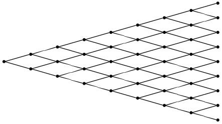
The resulting graph looks like the following:

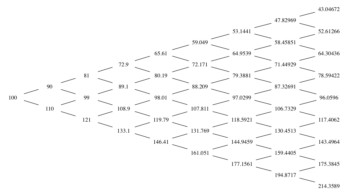
If we want to add labels to the lattice vertices, we can add the labels attribute:

[source lang=”R”]
> x<-capture.output(dotlattice(genlattice(N=8, u=1.1, d=0.9), labels=TRUE))
> cat(x, file="/tmp/lattice1.dot")
[/source]