Category: Coding

In the first two parts of this series, I looked at the basics of the interface I created between rmathlib and kdb+. In this post, I’ll go through some of the convenience functions I wrote to emulate some basic R functionality.

NOTE: I wrote these functions as a learning exercise to familiarise myself with q/kdb+ a bit more – they are very simplistic and I am sure there are much better ways to do them (I know the very nice qml project does a lot of this stuff, plus interfaces to external BLAS libraries).

Some basics: load the library:

q)\l rmath.q

seq – sequence function

The first convenience function is seq, which is like R’s seq() or Numpy’s arange() in that it takes a start and end point, and generates a range of numbers.

q)seq[1;100]
1 2 3 4 5 6 7 8 9 10 11 12 13 14 15 16 17 18 19 20 21 22 23 24 25 26...

The function is just a curried wrapper around seqn, which also takes a step size:

q)seqn[1;10;.5]
1 1.5 2 2.5 3 3.5 4 4.5 5 5.5 6 6.5 7 7.5 8 8.5 9 9.5 10

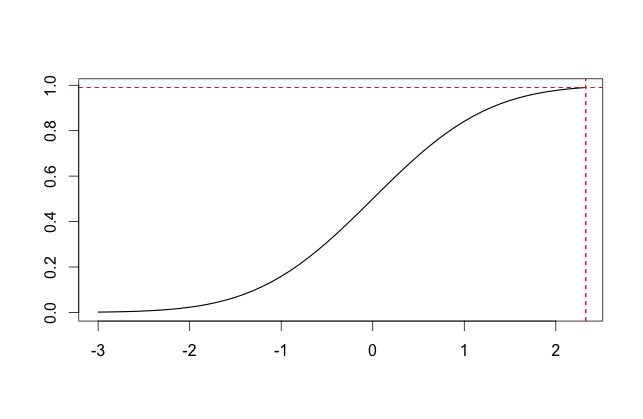
This is handy when working with some of the probability generation functions shown last time. For instance the commands below calculate the normal distribution (cdf) values for evenly spaced points from -3 to 3:

q)each[{pnorm[x;0;1]}] seqn[-3;3;.5]
0.001349898 0.006209665 0.02275013 0.0668072...

table – Symbol Tabulation

R provides a handy function to show summary count tables of factor levels. In q, this can be used as follows:

q)t:([] sym:1000?`A`B`C`D)
q)table[`sym;t]
B| 241
A| 244
C| 256
D| 259

This tabulates the column sym from the table t. The summary is ordered by increasing frequency count.

NOTE: this has really no advantage over the standard

q)`x xasc select count i by sym from t
sym| x  
---| ---
B  | 241
A  | 244
C  | 256
D  | 259

except some slight brevity.

range – Min/Max

The range function simply returns the boundaries of a set of values:

q)x:rnorm[10000]
q)range[x]
-3.685814 4.211363
q)abs (-) . range[x]   / absolute range 
7.897177

summary – Min/Max/Mean/Median/IQR

The summary function provides summary stats, a la R’s summary() function:

q)x:norm[10000;3;2]
q)summary x
min   | -4.755305
1q    | 1.59379
median| 2.972523
mean  | 2.966736
3q    | 4.336589
max   | 10.00284

quantile – Quantile Calculations

A very simple quantile calc:

q)x:norm[10000;3;2]
q)quantile[x;.5]
2.973137

hist – Bin Count

Very crude bin count – specify the data and the number of bins:

q)hist[x;10]
-4.919383| 14
-3.279589| 101
-1.639794| 601
0        | 1856
1.639794 | 3043
3.279589 | 2696
4.919383 | 1329
6.559177 | 319
8.198972 | 40
9.838766 | 1

diag – Identity Matrix Generation

q)diag 10
1 0 0 0 0 0 0 0 0 0
0 1 0 0 0 0 0 0 0 0
0 0 1 0 0 0 0 0 0 0
0 0 0 1 0 0 0 0 0 0
0 0 0 0 1 0 0 0 0 0
0 0 0 0 0 1 0 0 0 0
0 0 0 0 0 0 1 0 0 0
0 0 0 0 0 0 0 1 0 0
0 0 0 0 0 0 0 0 1 0
0 0 0 0 0 0 0 0 0 1

Scale functions

Sometimes its very useful to scale an input data set – e.g. when feeding multiple inputs into a statistical model, large differences between the relative scales of the inputs combined with finite-precision computer arithmetic can result in some inputs being dwarfed by others. The scale function just adjusts the input as follows: \(X_{s}=(X-\mu)/\sigma\).

The example below scales two inputs with different ranges:

q)x:norm[10;0;1]; y:norm[10;5;3]
q)x
1.920868 -1.594028 -0.02312519 1.079606 -0.5310111 0.2762119 0.1218428 0.9584264 -0.4244091 -0.7981221
q)y
10.69666 2.357529 8.93505 3.65696 5.218461 3.246216 5.971919 7.557135 1.412827 1.246241
q)range x
-1.594028 1.920868
q)range y
1.246241 10.69666
q)range scale x
-1.74507 1.878671
q)range scale y
-1.232262 1.845551

There are other useful scaling measures, including the min/max scale: \( \frac{x-min(x)}{max(x)-min(x)} \). This is implemented using the minmax function:

q)minmax x
1 0 0.4469273 0.760658 0.302432 0.5320897 0.4881712 0.726182 0.3327606 0.226438
range minmax x
0 1f

There are other functions which are useful for scaling, e.g. the RMSD (root-mean-square deviation): \( \sqrt{\frac{\sum{x_i^2}}{N}}\):

q)x:rnorm 1000
q)rms x
1.021065

nchoosek – Combinations

The nchoosek function calculates the number of combinations of N items chosen k at a time (i.e. \({N}\choose{k}\):

q)nchoosek[100;5]
7.528752e+07
q)each[{nchoosek[10;x]}] seq[1;10]
10 45 120 210 252 210 120 45 10 1f

The source file is available here: https://github.com/rwinston/kdb-rmathlib/blob/master/rmath_aux.q.

Following on from the last post on integrating some rmathlib functionality with kdb+, here is a sample walkthrough of how some of the functionality can be used, including some of the R-style wrappers I wrote to emulate some of the most commonly-used R commands in q.

Loading the rmath library

Firstly, load the rmathlib library interface:

q)\l rmath.q

Random Number Generation

R provides random number generation facilities for a number of distributions. This is provided using a single underlying uniform generator (R provides many different RNG implementations, but in the case of Rmathlib it uses a Marsaglia-multicarry type generator) and then uses different techniques to generate numbers distributed according to the selected distribution. The standard technique is inversion, where a uniformly distributed number in [0,1] is mapped using the inverse of the probability distribution function to a different distribution. This is explained very nicely in the book “Non-Uniform Random Variate Generation”, which is availble in full here: http://luc.devroye.org/rnbookindex.html.

In order to make random variate generation consistent and reproducible across R and kdb+, we need to be able to seed the RNG. The default RNG in rmathlib takes two integer seeds. We can set this in an R session as follows:

[source lang=”R”]
> .Random.seed[2:3]<-as.integer(c(123,456))
[/source]

and the corresponding q command is:

q)sseed[123;456]

Conversely, getting the current seed value can be done using:

q)gseed[]
123 456i

The underlying uniform generator can be accessed using runif:

q)runif[100;3;4]
3.102089 3.854157 3.369014 3.164677 3.998812 3.092924 3.381564 3.991363 3.369..

produces 100 random variates uniformly distributed between [3,4].

Then for example, normal variates can be generated:

q)rnorm 10
-0.2934974 -0.334377 -0.4118473 -0.3461507 -0.9520977 0.9882516 1.633248 -0.5957762 -1.199814 0.04405314

This produces identical results in R:

[source lang=”r”]
> rnorm(10)
[1] -0.2934974 -0.3343770 -0.4118473 -0.3461507 -0.9520977 0.9882516 1.6332482 -0.5957762 -1.1998144
[10] 0.0440531
[/source]

Normally-distributed variables with a distribution of \( N(\mu,\sigma) \) can also be generated:

q)dev norm[10000;3;1.5]
1.519263
q)avg norm[10000;3;1.5]
2.975766

Or we can alternatively scale a standard normal \( X ~ N(0,1) \) using \( Y = \sigma X + \mu \):

q)x:rnorm[1000]
q) `int$ (avg x; dev x)
0 1i
q)y:(x*3)+5
q) `int$ (avg y; dev y)
5 3i

Probability Distribution Functions

As well as random variate generation, rmathlib also provides other functions, e.g. the normal density function:

q)dnorm[0;0;1]
0.3989423

computes the normal density at 0 for a standard normal distribution. The second and third parameters are the mean and standard deviation of the distribution.

The normal distribution function is also provided:

q)pnorm[0;0;1]
0.5

computes the distribution value at 0 for a standard normal (with mean and standard deviation parameters).

Finally, the quantile function (the inverse of the distribution function – see the graph below – the quantile value for .99 is mapped onto the distribution function value at that point: 2.32):

q)qnorm[.99;0;1]
2.326348

We can do a round-trip via pnorm() and qnorm():

q)`int $ qnorm[ pnorm[3;0;1]-pnorm[-3;0;1]; 0; 1]
3i

Thats it for the distribution functions for now – rmathlib provides lots of different distributions (I have just linked in the normal and uniform functions for now. There are some other functions that I have created that I will cover in a future post.

All code is on github: https://github.com/rwinston/kdb-rmathlib

[Check out part 3 of this series]