Following on from the last post on integrating some rmathlib functionality with kdb+, here is a sample walkthrough of how some of the functionality can be used, including some of the R-style wrappers I wrote to emulate some of the most commonly-used R commands in q.
Loading the rmath library
Firstly, load the rmathlib library interface:
q)\l rmath.q
Random Number Generation
R provides random number generation facilities for a number of distributions. This is provided using a single underlying uniform generator (R provides many different RNG implementations, but in the case of Rmathlib it uses a Marsaglia-multicarry type generator) and then uses different techniques to generate numbers distributed according to the selected distribution. The standard technique is inversion, where a uniformly distributed number in [0,1] is mapped using the inverse of the probability distribution function to a different distribution. This is explained very nicely in the book “Non-Uniform Random Variate Generation”, which is availble in full here: http://luc.devroye.org/rnbookindex.html.
In order to make random variate generation consistent and reproducible across R and kdb+, we need to be able to seed the RNG. The default RNG in rmathlib takes two integer seeds. We can set this in an R session as follows:
[source lang=”R”]
> .Random.seed[2:3]<-as.integer(c(123,456))
[/source]
and the corresponding q command is:
q)sseed[123;456]
Conversely, getting the current seed value can be done using:
q)gseed[]

123 456i
The underlying uniform generator can be accessed using runif:
q)runif[100;3;4]

3.102089 3.854157 3.369014 3.164677 3.998812 3.092924 3.381564 3.991363 3.369..
produces 100 random variates uniformly distributed between [3,4].
Then for example, normal variates can be generated:
q)rnorm 10

-0.2934974 -0.334377 -0.4118473 -0.3461507 -0.9520977 0.9882516 1.633248 -0.5957762 -1.199814 0.04405314
This produces identical results in R:
[source lang=”r”]
> rnorm(10)
[1] -0.2934974 -0.3343770 -0.4118473 -0.3461507 -0.9520977 0.9882516 1.6332482 -0.5957762 -1.1998144
[10] 0.0440531
[/source]
Normally-distributed variables with a distribution of \( N(\mu,\sigma) \) can also be generated:
q)dev norm[10000;3;1.5]

1.519263

q)avg norm[10000;3;1.5]

2.975766
Or we can alternatively scale a standard normal \( X ~ N(0,1) \) using \( Y = \sigma X + \mu \):
q)x:rnorm[1000]

q) `int$ (avg x; dev x)

0 1i

q)y:(x*3)+5

q) `int$ (avg y; dev y)

5 3i
Probability Distribution Functions
As well as random variate generation, rmathlib also provides other functions, e.g. the normal density function:
q)dnorm[0;0;1]

0.3989423
computes the normal density at 0 for a standard normal distribution. The second and third parameters are the mean and standard deviation of the distribution.
The normal distribution function is also provided:
q)pnorm[0;0;1]

0.5
computes the distribution value at 0 for a standard normal (with mean and standard deviation parameters).
Finally, the quantile function (the inverse of the distribution function – see the graph below – the quantile value for .99 is mapped onto the distribution function value at that point: 2.32):
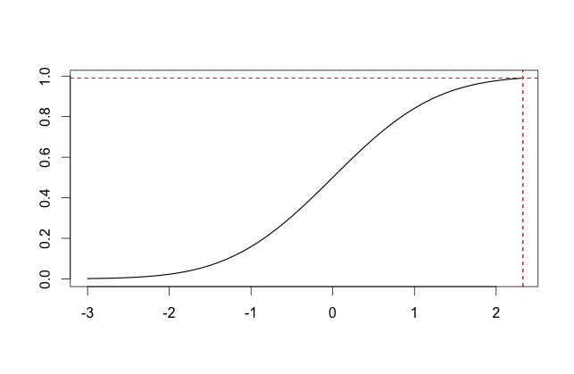
q)qnorm[.99;0;1]

2.326348
We can do a round-trip via pnorm() and qnorm():
q)`int $ qnorm[ pnorm[3;0;1]-pnorm[-3;0;1]; 0; 1]

3i
Thats it for the distribution functions for now – rmathlib provides lots of different distributions (I have just linked in the normal and uniform functions for now. There are some other functions that I have created that I will cover in a future post.
All code is on github: https://github.com/rwinston/kdb-rmathlib
[Check out part 3 of this series]