The Mandelbrot Set is possibly one of the most visually appealing mathematical visualizations. The set is defined as the set of complex numbers $c$ for which the function $f_c(z) = z^2 + c$ remains bounded when iterated – i.e. the sequence $f_c(z), f_c(f_c(z)),f_c(f_c(f_c(…)))$ remains bounded below some fixed absolute threshold.
The basic method to generate a simple Mandelbrot set is fairly simple:
- Choose the values of $c$ to put in the iteration $z\rightarrow z^2+c$;
- Iteratively apply the mapping for each value of $c$ and test if the updated value is now $\geq \epsilon$ where $\epsilon$ is some fixed absolute threshold;
- Update our output grid to reflect the intensity at point $c$ – this can be a simple 1/0 to indicate that the iteration has become unbounded (or ‘escaped’) or it can be a value reflecting how many iterations it took before the value was determined to escape (or not)
R has a ‘native’ representation for complex numbers but for this example we will just use a 2-element vector as a complex number representation, each element being the real and imaginary components respectively.
The iterative step at each point to update the current value of $z \rightarrow z^2+c$ is computed as follows – if $z$ is assumed to be a complex number of the form $x+yi$:
$$(x+yi)(x+yi) = x^2-y^2+2xyi$$
So $Re(z)\rightarrow x^2-y^2+Re(c) $ and $Im(z) \rightarrow 2xy+Im(c)$
Here is some simple R code to illustrate:
# Subset of x-y plane
x <- c(-2,1)
y <- c(-1.5, 1.5)

# Number of points in each dimension
nx <- 500
ny <- 500

xgrid <- seq(x[1],x[2], length.out = nx)
ygrid <- seq(y[1],y[2], length.out = ny)


mand <- function(xgrid,ygrid,frac) {
  i <- j <- it <- 1
  z <- c <- zprev <- c(0,0)
  TOL <- 4  # Escape value
  N <- 50   # Number of iterations to test for escape
  # The output fractal trace
  frac <- matrix(nrow=nx, ncol=ny, byrow=TRUE)

  for (i in seq_along(xgrid)) {
    for (j in seq_along(ygrid)) {
      c <- c(xgrid[i],ygrid[j])
      z <- c(0,0)

      for (k in 1:N) {
        it <- k
        zprev <- z
        # If zprev is a complex number x + yi
        # Then we update z as follows:
        # Re(z) <- (x^2-y^2) + Re(c)
        z[1] <- zprev[1]*zprev[1]-zprev[2]*zprev[2]+c[1]
        # Im(z) <- 2*z*y + Im(c)
        z[2] <- 2*zprev[1]*zprev[2]+c[2]
        if ((z[1]*z[1] + z[2]*z[2])>TOL) { break }
      }
      frac[i,j] <- it
    }
  }

  return(list(x=xgrid,y=ygrid,z=frac))
}
To call the function and plot the output:
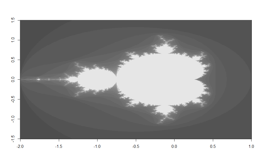
m <- mand(xgrid,ygrid,frac)
image(m, col=gray.colors(50))
Which should produce an image like the following:
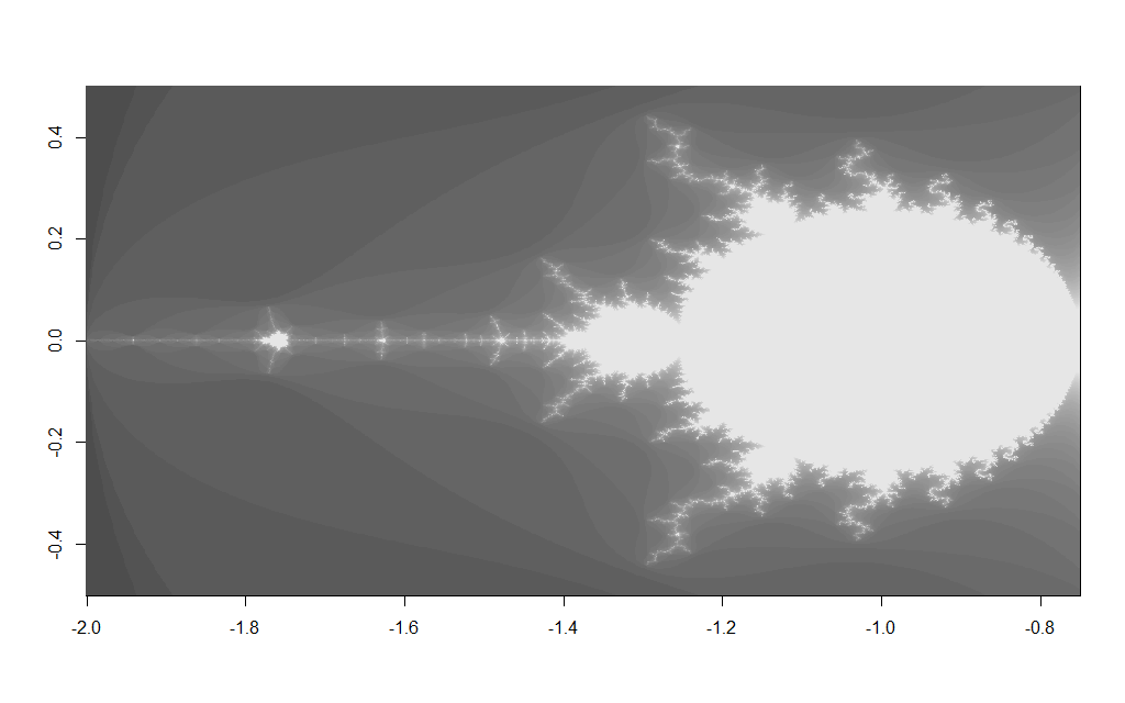
Changing the $x$ and $y$ grid coordinates enables you too zoom in to various areas on the fractal e.g. changing the x/y grid to:
x <- c(-2,-0.75)
y <- c(-0.5, 0.5)
Results in the image below
The main drawback of iterative plain R code like this is that it is slow – however this could be speeded up using a native interface e.g. Rcpp and computing the iterative process in C/C++ code, where some of the copying overhead may be avoided.