Categories
Finance R Statistics

Density Estimation of High-Frequency Financial Data

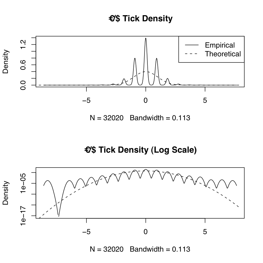
Frequently we will want to estimate the empirical probability density function of real-world data and compare it to the theoretical density from one or more probability distributions. The following example shows the empirical and theoretical normal density for EUR/USD high-frequency tick data \(X\) (which has been transformed using log-returns and normalized via \(\frac{X_i-\mu_X}{\sigma_X}\)). The theoretical normal density is plotted over the range \(\left(\lfloor\mathrm{min}(X)\rfloor,\lceil\mathrm{max}(X)\rceil\right)\). The results are in the figure below. The discontinuities and asymmetry of the discrete tick data, as well as the sharp kurtosis and heavy tails (a corresponding interval of \(\approx \left[-8,+7\right]\) standard deviations away from the mean) are apparent from the plot.
tick density
Empirical and Theoretical Tick Density

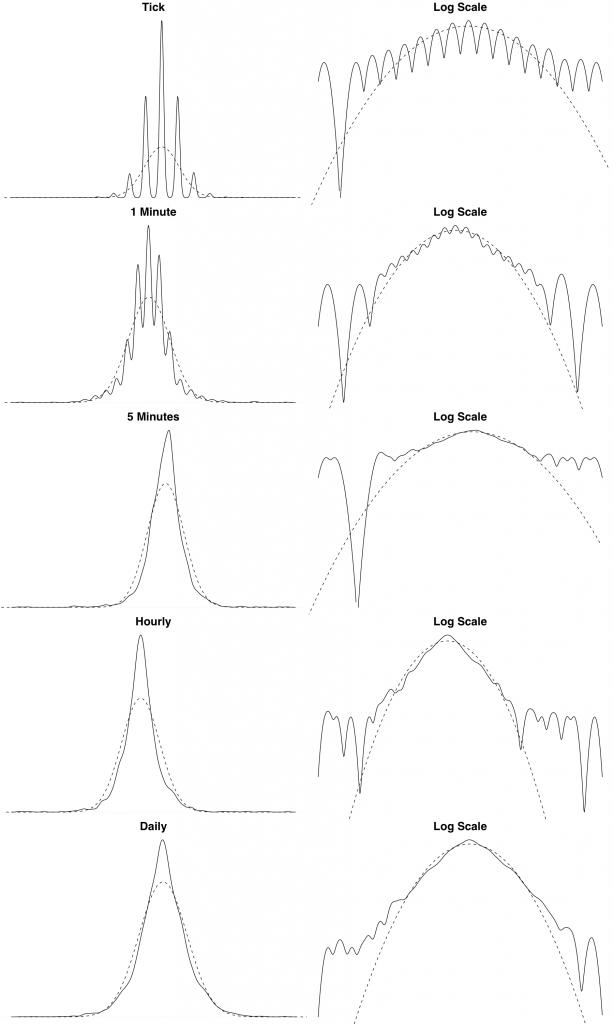
We also show the theoretical and empirical density for the EUR/USD exchange rate log returns over different timescales. We can see from these plots that the distribution of the log returns seems to be asymptotically converging to normality. This is a typical empirical property of financial data.
density_scaled
Density Estimate Across Varying Timescales

The following R source generates empirical and theoretical density plots across different timescales. The data is loaded from files that are sampled at different intervals. I cant supply the data unfortunately, but you should get the idea.

[source lang=”R”]
# Function that reads Reuters CSV tick data and converts Reuters dates
# Assumes format is Date,Tick
readRTD <- function(filename) {
tickData <- read.csv(file=filename, header=TRUE, col.names=c("Date","Tick"))
tickData$Date <- as.POSIXct(strptime(tickData$Date, format="%d/%m/%Y %H:%M:%S"))
tickData
}

# Boilerplate function for Reuters FX tick data transformation and density plot
plot.reutersFXDensity <- function() {
filenames <- c("data/eur_usd_tick_26_10_2007.csv",
"data/eur_usd_1min_26_10_2007.csv",
"data/eur_usd_5min_26_10_2007.csv",
"data/eur_usd_hourly_26_10_2007.csv",
"data/eur_usd_daily_26_10_2007.csv")
labels <- c("Tick", "1 Minute", "5 Minutes", "Hourly", "Daily")

par(mfrow=c(length(filenames), 2),mar=c(0,0,2,0), cex.main=2)
tickData <- c()
i <- 1
for (filename in filenames) {
tickData[[i]] <- readRTD(filename)
# Transform: `$Y = \nabla\log(X_i)$`
logtick <- diff(log(tickData[[i]]$Tick))
# Normalize: `$\frac{(Y-\mu_Y)}{\sigma_Y}$`
logtick <- (logtick-mean(logtick))/sd(logtick)
# Theoretical density range: `$\left[\lfloor\mathrm{min}(Y)\rfloor,\lceil\mathrm{max}(Y)\rceil\right]$`
x <- seq(floor(min(logtick)), ceiling(max(logtick)), .01)
plot(density(logtick), xlab="", ylab="", axes=FALSE, main=labels[i])
lines(x,dnorm(x), lty=2)
#legend("topleft", legend=c("Empirical","Theoretical"), lty=c(1,2))
plot(density(logtick), log="y", xlab="", ylab="", axes=FALSE, main="Log Scale")
lines(x,dnorm(x), lty=2)
i <- i + 1
}
par(op)
}
[/source]
Categories
Coding Finance R Statistics

Binomial Pricing Trees in R

Binomial Tree Simulation

The binomial model is a discrete grid generation method from \(t=0\) to \(T\). At each point in time (\(t+\Delta t\)) we can move up with probability \(p\) and down with probability \((1-p)\). As the probability of an up and down movement remain constant throughout the generation process, we end up with a recombining binary tree, or binary lattice. Whereas a balanced binomial tree with height \(h\) has \(2^{h+1}-1\) nodes, a binomial lattice of height \(h\) has \(\sum_{i=1}^{h}i\) nodes.

The algorithm to generate a binomial lattice of \(M\) steps (i.e. of height \(M\)) given a starting value \(S_0\), an up movement \(u\), and down movement \(d\), is:


FOR i=1 to M
FOR j=0 to i
STATE S(j,i) = S(0)*u^j*d^(n-j)
ENDFOR
ENDFOR

We can write this function in R and generate a graph of the lattice. A simple lattice generation function is below:

[source lang=”R”]
# Generate a binomial lattice
# for a given up, down, start value and number of steps
genlattice <- function(X0=100, u=1.1, d=.75, N=5) {
X <- c()
X[1] <- X0
count <- 2

for (i in 1:N) {
for (j in 0:i) {
X[count] <- X0 * u^j * d^(i-j)
count <- count + 1
}
}
return(X)
}
[/source]

We can generate a sample lattice of 5 steps using symmetric up-and-down values:

[source lang=”R”]
> genlattice(N=5, u=1.1, d=.9)
[1] 100.000 90.000 110.000 81.000 99.000 121.000 72.900 89.100 108.900 133.100 65.610
[12] 80.190 98.010 119.790 146.410 59.049 72.171 88.209 107.811 131.769 161.051
[/source]

In this case, the output is a vector of alternate up and down state values.

We can nicely graph a binomial lattice given a tool like graphviz, and we can easily create an R function to generate a graph specification that we can feed into graphviz:

[source lang=”R”]
function(S, labels=FALSE) {
shape <- ifelse(labels == TRUE, "plaintext", "point")

cat("digraph G {", "\n", sep="")
cat("node[shape=",shape,", samehead, sametail];","\n", sep="")
cat("rankdir=LR;","\n")

cat("edge[arrowhead=none];","\n")

# Create a dot node for each element in the lattice
for (i in 1:length(S)) {
cat("node", i, "[label=\"", S[i], "\"];", "\n", sep="")
}

# The number of levels in a binomial lattice of length N
# is `$\frac{\sqrt{8N+1}-1}{2}$`
L <- ((sqrt(8*length(S)+1)-1)/2 – 1)

k<-1
for (i in 1:L) {
tabs <- rep("\t",i-1)
j <- i
while(j>0) {
cat("node",k,"->","node",(k+i),";\n",sep="")
cat("node",k,"->","node",(k+i+1),";\n",sep="")
k <- k + 1
j <- j – 1
}
}

cat("}", sep="")
}
[/source]

This will simply output a dot script to the screen. We can capture this script and save it to a file by invoking:

[source lang=”R”]
> x<-capture.output(dotlattice(genlattice(N=8, u=1.1, d=0.9)))
> cat(x, file="/tmp/lattice1.dot")
[/source]

We can then invoke dot from the command-line on the generated file:

[source lang=”bash”]
$ dot -Tpng -o lattice.png -v lattice1.dot
[/source]

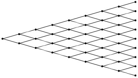
The resulting graph looks like the following:

Binomial Lattice
Binomial Lattice (no labels)

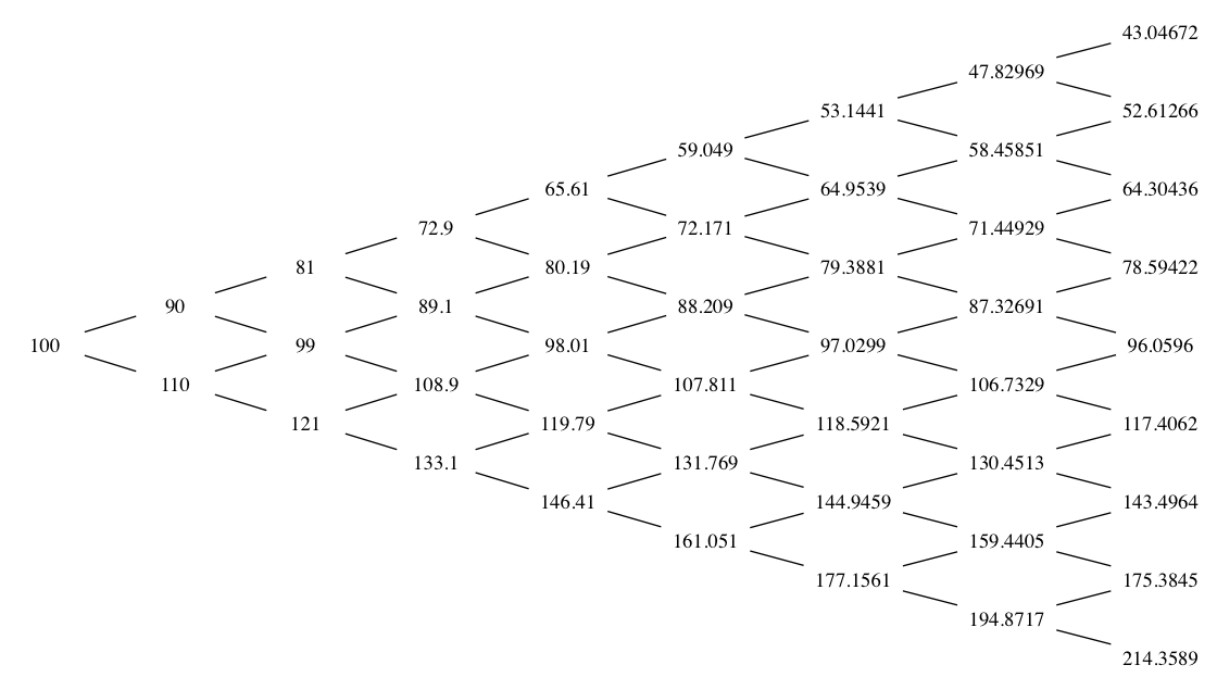
If we want to add labels to the lattice vertices, we can add the labels attribute:

[source lang=”R”]
> x<-capture.output(dotlattice(genlattice(N=8, u=1.1, d=0.9), labels=TRUE))
> cat(x, file="/tmp/lattice1.dot")
[/source]

Lattice (labels)
Binomial Lattice (labels)
Categories
Finance

Statistical Arbitrage II : Simple FX Arbitrage Models

In the context of the foreign exchange markets, there are several simple no-arbitrage conditions, which, if violated outside of the boundary conditions imposed by transaction costs, should provide the arbitrageur with a theoretical profit when market conditions converge to theoretical normality.

Detection of arbitrage conditions in the FX markets requires access to high-frequency tick data, as arbitrage opportunities are usually short-lived. Various market inefficiency conditions exist in the FX markets. Apart from the basic strategies outlined in the following sections, other transient opportunities may exist, if the trader or trading system can detect and act on them quickly enough.

Round-Trip Arbitrage
Possibly the most well-known no-arbitrage boundary condition in foreign exchange is the covered interest parity condition. The covered interest parity condition is expressed as:

\[ (1+r_d) = \frac{1}{S_t}(1+r_f)F_t \]

which specifies that it should not be possible to earn positive return by borrowing domestic assets at $\(r_d\) for lending abroad at \(r_f\) whilst covering the exchange rate risk through a forward contract \(F_t\) of equal maturity.

Accounting for transaction costs, we have the following no-arbitrage relationships:

\[ (1+r_d^a) \geq \frac{1}{S^a}(1+r_f^b)F^b \]
\[ (1+r_f^b) \geq S^b(1+r_d^b)\frac{1}{F^a} \]

For example, the first condition states that the cost of borrowing domestic currency at the ask rate (\(1+r_d^a\)) should be at least equal to the cost of converting said currency into foreign currency (\(\frac{1}{s^a}\)) at the prevailing spot rate \(S^a\) (assuming that the spot quote \(S^a\) represents the cost of a unit of domestic currency in terms of foreign currency), invested at \(1+r_f^b\), and finally converted back into domestic currency via a forward trade at the ask rate (\(F^a\)). If this condition is violated, then we can perform round-trip arbitrage by converting, investing, and re-converting at the end of the investment term. Persistent violations of this condition are the basis for the roaring carry trade, in particular between currencies such as the Japanese Yen and higher yielding currencies such as the New Zealand dollar and the Euro.

Triangular Arbitrage
A reduced form of FX market efficiency is that of triangular arbitrage, which is the geometric relationship between three currency pairs. Triangular arbitrage is defined in two forms, forward arbitrage and reverse arbitrage. These relationships are defined below.

$$ \left(\frac{C_1}{C_2}\right)_{ask} \left(\frac{C_2}{C_3}\right)_{ask} = \left(\frac{C_1}{C_3}\right)_{bid} \\
\left(\frac{C_1}{C_2}\right)_{bid} \left(\frac{C_2}{C_3}\right)_{bid} = \left(\frac{C_1}{C_3}\right)_{ask} $$

With two-way high-frequency prices, we can simultaneously calculate the presence of forward and reverse arbitrage.

A contrived example follows: if we have the following theoretical two-way tradeable prices: \(\left(\frac{USD}{JPY}\right) = 90/110\), \(\left(\frac{GBP}{USD}\right) = 1.5/1.8\), and \(\left(\frac{JPY}{GBP}\right) = 150/200\). By the principle of triangular arbitrage, the theoretical two-way spot rate for JPY/GBP should be \(135/180\). Hence, we can see that JPY is overvalued relative to GBP. We can take advantage of this inequality as follows, assuming our theoretical equity is 1 USD:

  • Pay 1 USD and receive 90 JPY ;
  • Sell 90 JPY ~ and receive \(\left(\frac{90}{135}\right)\) GBP ;
  • Pay \(\left(\frac{90}{135}\right)\) GBP, and receive \(\left(\frac{90}{135}\right) \times \) 1.5 USD = 1.32 USD.

We can see that reverse triangular arbitrage can detect a selling opportunity (i.e. the bid currency is overvalued), whilst forward triangular arbitrage can detect a buying opportunity (the ask currency is undervalued).

The list of candidate currencies could be extended, and the arbitrage condition could be elegantly represented by a data structure called a directed graph. This would involve creating an adjacency matrix \(R\), in which an element \(R_{i,j}\) contains a measure representing the cost of transferring between currency \(i\) and currency \(j\).

Triangular Graph

Estimating Position Risk
When executing an arbitrage trade, there are some elements of risk. An arbitrage trade will normally involve multiple legs which must be executed simultaneously and at the specified price in order for the trade to be successful. As most arbitrage trades capitalize on small mispricings in asset values, and rely on large trading volumes to achieve significant profit, even a minor movement in the execution price can be disastrous. Hence, a trading algorithm should allow for both trading costs and slippage, normally by adding a margin to the profitability ratio. The main risk in holding an FX position is related to price slippage, and hence, the variance of the currency that we are holding.