Here is a toy example of implementing Newton’s method in R. I found some old code that I had written a few years ago when illustrating the difference between convergence properties of various root-finding algorithms, and this example shows a couple of nice features of R.
Newtons method is an iterative root-finding algorithm where we start with an initial guess \(x_0\) and each successive guess is refined using the iterative process:
$$ x_{n+1} = x_n – \frac{f(x_n)}{f'(x_n)} $$
Here is a simple implementation of this in R:
[source lang=”R”]
newton <- function(f, tol=1E-12,x0=1,N=20) {
h <- 0.001
i <- 1; x1 <- x0
p <- numeric(N)
while (i<=N) {
df.dx <- (f(x0+h)-f(x0))/h
x1 <- (x0 – (f(x0)/df.dx))
p[i] <- x1
i <- i + 1
if (abs(x1-x0) < tol) break
x0 <- x1
}
return(p[1:(i-1)])
}
[/source]
Note a couple of things:
* The step-size for numerical differentiation is hardcoded to be 0.001. This is arbitrary and should probably be a parameter.
* The algorithm will run until either the number of steps N has been reached, or the error tolerance \(\left|x_{n+1}-x_n\right|< \epsilon\), where \(\epsilon\) is defined as the tolerance parameter tol.
* The function returns a vector of the iterated x positions, which will be <= N.
Here is a simple example: for instance, to find the zeros of the function
$$ f(x) = x^3 + 4x^2 - 10 $$
which in R we can represent as:
[source lang="R"]f <- function(x) { x^3 + 4*x^2 -10 }[/source]
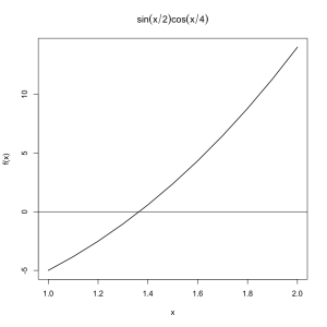
Let's plot the function over the range [1,2]:

[source lang=”R”]
plot(x,f(x), type=’l’, lwd=1.5, main=expression(sin(x/2) * cos(x/4)))
abline(h=0)
[/source]
It seems obvious from the plot that the zero of f(x) in the range [1,2] is somewhere between x=1.3 and x=1.4.
This is made even more clear if we tabulate the x,y values over this range:
[source lang=”R”]
> xy <- cbind(x,f(x))
> xy
x
[1,] 1.0 -5.000
[2,] 1.1 -3.829
[3,] 1.2 -2.512
[4,] 1.3 -1.043
[5,] 1.4 0.584
[6,] 1.5 2.375
[7,] 1.6 4.336
[8,] 1.7 6.473
[9,] 1.8 8.792
[10,] 1.9 11.299
[11,] 2.0 14.000
[/source]
Using the function defined earlier, we can run the root-finding algorithm:
[source lang=”R”]
> p <- newton(f, x0=1, N=10)
> p
[1] 1.454256 1.368917 1.365238 1.365230 1.365230 1.365230 1.365230
[/source]
This returns 1.365230 as the root of f(x). Plotting the last value in the iteration:

[source lang=”R”]
> abline(v=p[length(p)])
[/source]
In the iteration loop, we use a schoolbook-style numerical derivative:
$$ \frac{dy}{dx} = \frac{f(x+\epsilon)-f(x)}{\epsilon} $$
Its also worth noting that R has some support for symbolic derivatives, so we could use a symbolic function expression. A simple example of symbolic differentiation in R (note that R works with expression instances when using symbolic differentiation):
[source lang=”R”]
> e <- expression(sin(x/2)*cos(x/4))
> dydx <- D(e, "x")
> dydx
cos(x/2) * (1/2) * cos(x/4) – sin(x/2) * (sin(x/4) * (1/4))
[/source]
In order for this to be useful, obviously we need to be able to evaluate the calculated derivative. We can do this using eval:
[source lang=”R”]
> z <- seq(-1,1,.1)
> eval(dydx, list(x=z))
[1] 0.3954974 0.4146144 0.4320092 0.4475873 0.4612640 0.4729651 0.4826267
[8] 0.4901964 0.4956329 0.4989067 0.5000000 0.4989067 0.4956329 0.4901964
[15] 0.4826267 0.4729651 0.4612640 0.4475873 0.4320092 0.4146144 0.3954974
[/source]
Note that we can bind the x parameter in the expression when calling eval().

