Binomial Tree Simulation
The binomial model is a discrete grid generation method from \(t=0\) to \(T\). At each point in time (\(t+\Delta t\)) we can move up with probability \(p\) and down with probability \((1-p)\). As the probability of an up and down movement remain constant throughout the generation process, we end up with a recombining binary tree, or binary lattice. Whereas a balanced binomial tree with height \(h\) has \(2^{h+1}-1\) nodes, a binomial lattice of height \(h\) has \(\sum_{i=1}^{h}i\) nodes.
The algorithm to generate a binomial lattice of \(M\) steps (i.e. of height \(M\)) given a starting value \(S_0\), an up movement \(u\), and down movement \(d\), is:
FOR i=1 to M

FOR j=0 to i

 STATE S(j,i) = S(0)*u^j*d^(n-j)

ENDFOR

ENDFOR
We can write this function in R and generate a graph of the lattice. A simple lattice generation function is below:
[source lang=”R”]
# Generate a binomial lattice
# for a given up, down, start value and number of steps
genlattice <- function(X0=100, u=1.1, d=.75, N=5) {
X <- c()
X[1] <- X0
count <- 2
for (i in 1:N) {
for (j in 0:i) {
X[count] <- X0 * u^j * d^(i-j)
count <- count + 1
}
}
return(X)
}
[/source]
We can generate a sample lattice of 5 steps using symmetric up-and-down values:
[source lang=”R”]
> genlattice(N=5, u=1.1, d=.9)
[1] 100.000 90.000 110.000 81.000 99.000 121.000 72.900 89.100 108.900 133.100 65.610
[12] 80.190 98.010 119.790 146.410 59.049 72.171 88.209 107.811 131.769 161.051
[/source]
In this case, the output is a vector of alternate up and down state values.
We can nicely graph a binomial lattice given a tool like graphviz, and we can easily create an R function to generate a graph specification that we can feed into graphviz:
[source lang=”R”]
function(S, labels=FALSE) {
shape <- ifelse(labels == TRUE, "plaintext", "point")
cat("digraph G {", "\n", sep="")
cat("node[shape=",shape,", samehead, sametail];","\n", sep="")
cat("rankdir=LR;","\n")
cat("edge[arrowhead=none];","\n")
# Create a dot node for each element in the lattice
for (i in 1:length(S)) {
cat("node", i, "[label=\"", S[i], "\"];", "\n", sep="")
}
# The number of levels in a binomial lattice of length N
# is `$\frac{\sqrt{8N+1}-1}{2}$`
L <- ((sqrt(8*length(S)+1)-1)/2 – 1)
k<-1
for (i in 1:L) {
tabs <- rep("\t",i-1)
j <- i
while(j>0) {
cat("node",k,"->","node",(k+i),";\n",sep="")
cat("node",k,"->","node",(k+i+1),";\n",sep="")
k <- k + 1
j <- j – 1
}
}
cat("}", sep="")
}
[/source]
This will simply output a dot script to the screen. We can capture this script and save it to a file by invoking:
[source lang=”R”]
> x<-capture.output(dotlattice(genlattice(N=8, u=1.1, d=0.9)))
> cat(x, file="/tmp/lattice1.dot")
[/source]
We can then invoke dot from the command-line on the generated file:
[source lang=”bash”]
$ dot -Tpng -o lattice.png -v lattice1.dot
[/source]
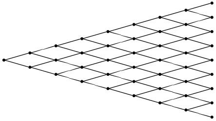
The resulting graph looks like the following:

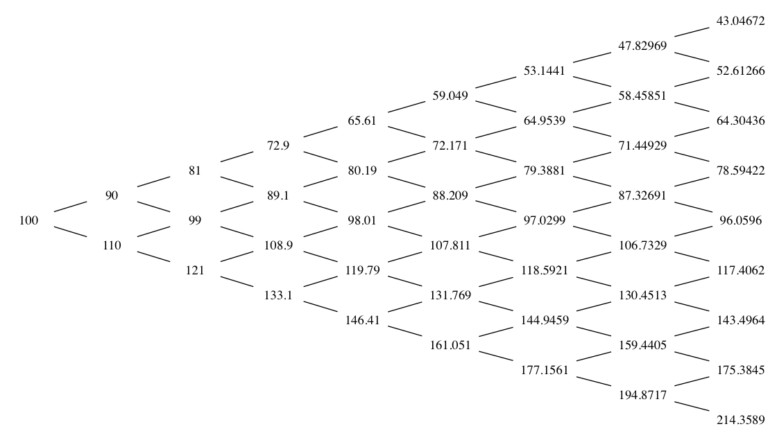
If we want to add labels to the lattice vertices, we can add the labels attribute:
[source lang=”R”]
> x<-capture.output(dotlattice(genlattice(N=8, u=1.1, d=0.9), labels=TRUE))
> cat(x, file="/tmp/lattice1.dot")
[/source]
